Myron is not intended to be a programming language, but recursion and piecewise
functions provide some aspects of a functional programming language.
A function is said to be
recursive when it references itself directly or indirectly.
If a piecewise function provides a base piece and at least one other
piece that reduces other cases towards the base piece by calling the
function directly or indirectly, the function is
said to have recursive termination. Several examples of recursive piecewise
functions are given here.
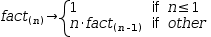
9.3.1 Factorial
The
factorial
operator is defined as
n !=n⋅(n-1) !
for integers
n>1, and 1 for
n≤1. As a piecewise function, this can be written
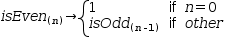
Mutual recursion
occurs when two functions are each defined in terms of the other. An
admittedly contrived example is given by functions that determine
evenness or oddness of an integer parameter by decrementing and
calling each other.
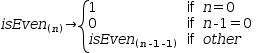
isEven(n)→n=0?1:isOdd(n-1)
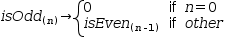
isOdd(n)→n=0?0:isEven(n-1)
Then
((isEven(n), isOdd(n))|n∈0, 3)
distributes and evaluates to
((1, 0), (0, 1), (1, 0), (0, 1)).
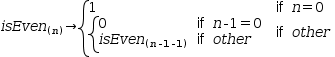
Mutual recursion can sometimes be converted to simple recursion by
inline expansion of one of the functions. In the example of isEven,
select
.{isOdd(n-1)}
and Substitute to produce the simple recursion
isEven(n)→n=0?1:(n-1=0?0:isEven(n-1-1)).
The elaboration of the latter function can be simplified to
isEven(n)→if(n=0→1, n-1=0→0, 1→isEven(n-1-1)).
9.3.3 Greatest Common Divisor
Euclid's
GCD
algorithm can be expressed as
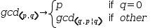
gcd(p, q)→q=0?p:gcd(q, p¦q).
Then
gcd(120, 93)
is 3.
To see what is happening during execution of the algorithm, it would
be useful to trace the recursive path of evaluation. The usual
techniques for tracing use some sort of “print” facility
or updates to an ever growing log variable. Myron has neither facility
but there is still a way. GCD can be rewritten as
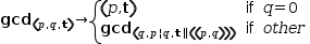
gcdʈ(p, q, tʈ)→q=0?(p, tʈ):gcdʈ(q, p¦q, tʈ‖(, (p, q))).
Then
gcdʈ(120, 93, (, ))
evaluates to
(3, ((120, 93), (93, 27), (27, 12), (12, 3))). The first element of the result tuple is the expected real result.
The second element is a tuple of tuples that trace the p and q
parameters through the recursion. The tracing technique can be applied
to any recursive function.
This example shows some of the subtleties of Myron's expression
language. Firstly, each branch of a piecewise function must have the
same expression type. Because the first branch is a tuple, the
function whose elaboration is the piecewise function must have a tuple
type. In turn, the function referenced recursively in the second
branch must also have a tuple type.
Secondly, the right argument of the concatenation operator in the
second branch is a singleton tuple, although it appears as a doubly
nested parenthesized expression. The singleton uses the notation
(,(p,q))
to appear as
(, (p, q)).
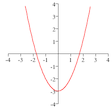
9.3.4 Newton's Method
Newton's method
for finding a root of function is an example of a function that
iterates to convergence. Here, convergence is achieved when the value
of the function approaches 0. The method is given by
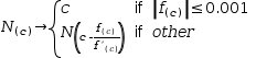
N(c)→|f(c)|≤0.001?c:N(c-f(c)÷f’(c))
.
Use of the function
N(c)
is illustrated by placing a definition
f(x)→x^2-3
and
f’(x)→2⋅x
in the workspace. A plot of
f(x)
in Figure
9.10
shows roots at approximately
±1.75.
N(-0.5)
and
N(0.5)
evaluate to
±1.73
(more precisely,
±1.7323080932066348, which is within one 1000th of the actual root.
Figure 9.10 A function with local minima
at 0
Written as a traceable function, Newton's method becomes
Then
Nʈ(0.5, (, ))
evaluates to
(1.73, (0.5, 3.25, 2.09, 1.76)).
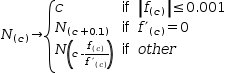
Newton's method won't converge if
f’(c)=0. Although Myron avoids infinite recursion by limiting the depth of
function calls, violating the limit does not produce a useful result.
A better way is to modify the piecewise function to “bump”
c when it falls on an local maxima or minima. Thus
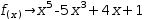
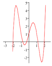
When using Newton's method for a function with multiple roots, it is
convenient to generate and then evaluate
N(c)
at several points. Such is the case for
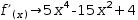
f(x)→x^5-5⋅x^3+4⋅x+1, shown in Figure
9.11, and it's derivative
f’(x)→5⋅x^4-15⋅x^2+4.
Figure 9.11
f(x)→x^5-5⋅x^3+4⋅x+1
A tuple with several initial guesses is given by
(N(r)|r∈-2, 2). Distributing this tuple and then evaluating it produces the roots
(, -2.04, -0.791, -0.276, 1.15, 1.95).
9.3.5 Quadrature
Quadrature
sums the areas of many small rectangles to approximate a definite
integral. It is sometimes used when an integral is not amenable to
symbolic manipulation. The integral
∫0, 1, x^2 ⅆx
is used here as an example and, because it simplifies to an exact
value,
1/3, it can be used to illustrate how well quadrature approximates a
definite integral.
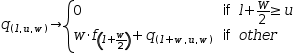
Using recursion, an approximation using quadrature can be written as
q(l, u, w)→l+w÷2≥u?0:w⋅f(l+w÷2)+q(l+w, u, w),
where l and u are the lower and upper bounds of the region to be
measured. The final parameter, w, is the width of each rectangle.
Then, with
f(x)→x^2
located in the workspace,
q(0, 1, 0.1)
evaluates to 0.3325,
q(0, 1, 0.01)
evaluates to 0.333325; and
q(0, 1, 0.001)
runs into Myron's recursion limit, a pragmatic restriction that limits
the usefulness of recursive functions.
However, all is not lost, A non recursive version of quadrature can be
written using a series generator.
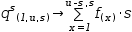
q__t(l, u, s)→(+|f_x∈(f(x)⋅s|x∈l, u-s, s))
uses a tuple generator nested within a generalized series generator to
sum the elements of a tuple, each of which is the area of a rectangle
beneath the function. Then
q__t(0, 1, 0.001)
evaluates to 0.333 (actually, 0.33283350000000034). The input form of
the series generator may prove instructive:
q__*(l,u,s)→(+|f_x∈(f(x)⋅s|x∈l,u-s,s)).
The expression can be written in a simpler way using a summation series generator.
q__s(l, u, s)→∑l, u-s, s, f(x)⋅sⅆx.